Efficiently computing eigenvalues and eigenvectors in Python

Let $M$ be an $n \times n$ matrix. A scalar $\lambda $ is an eigenvalue of $M$ if there is a non-zero vector $x$ (called eigenvector) s.t.:

$$M x = \lambda x$$

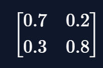
Eigenvalues and eigenvectors are crucial in many fields of science. For example, consider a discrete-time and discrete states Markov chain, whose transition matrix $M$ is defined as follows:

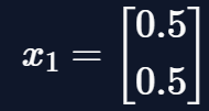
Let the initial state vector $x_1$ be:

We know that from $M$ and $x\_1$ we could compute all the successive states and it's true that:

$$x\_2 = M x \_1$$

$$x\_3 = M x\_2$$

and in general

$$x\k = M x\{k-1}$$

We may want to find a vector $x$ s.t.

$$Mx = x$$

Vectors with this property as known as steady-state vectors. It can be demonstrated that finding steady-state vectors equals finding any eigenvector $x$ with eigenvalue 1.

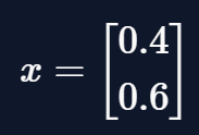
For example, the steady-state vector for the matrix $M$ is:

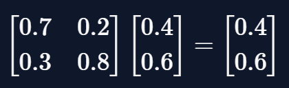
and one can easily show that

Finding eigenvalues and eigenvectors is not always easy to do by hand, and there are some algorithms to compute them. Unfortunately, this calculation may be expensive, especially with large matrices, and the result may be inaccurate due to approximations.

However, some algorithms perform better than others, and I want to discuss some of them in this article.

Solving characteristic equation

We can rewrite $M x = \lambda x$ as

$$M x-\lambda x = 0$$

$$( M-\lambda I)x = 0$$

This system has a non-trivial solution (i.e. $x \neq 0$) only if $det(M-\lambda I) =0$. $det(M-\lambda I) =0$ is known as the characteristic equation.

Expanding $det(M-\lambda I) =0$ we obtain a polynomial of degree $n$, whose roots are the eigenvalues of $M$. Computing eigenvectors from eigenvalues is trivial: for each eigenvalue $\lambda$, we just need to find the null space of the matrix $M-\lambda I$.

This is how we compute eigenvalues and eigenvectors by hand, but following this approach on a computer leads to some problems:

it depends on the computation of the determinant, which is a time-consuming process (due to the symbolic nature of the computation);
there is no formula for solving polynomial equations of degree higher than 4. Even though some techniques exist, like Newton's method, it's tough to find all the roots.

Therefore we need a different approach.

Iterative methods

Unfortunately, there is no simple algorithm to directly compute eigenvalues and eigenvectors for general matrices (there are special cases of matrices where it's possible, but I won't cover them in this article).

However, there are iterative algorithms that produce sequences that converge to eigenvectors or eigenvalues. There are several variations of these methods, I'll just cover two of them: the power method and the QR algorithm.

The power method

This method applies to matrices that have a dominant eigenvalue $\lambda\_d$ (i.e. an eigenvalue that is larger in absolute value than the other eigenvalues).

Let $M$ be an $n \times n$ matrix, the power method approximates a dominant eigenvector in the following steps:

$$x\_1 = Mx\_0$$

$$x\_2 = Mx\_1$$

$$x\k = Mx\{k-1}$$

And the more steps we take (i.e. the bigger $k$ is) the more accurate will be our approximation. This is expressed in the following formula

Once we have an approximation of the dominant eigenvector $x\_d$ we find the corresponding dominant eigenvalue $\lambda\_d$ with the Rayleigh quotient

$$\frac{(Mx)x}{xx} = \frac{(\lambda\_d x)x}{xx} = \frac{\lambda\_d (xx)}{xx}\lambda\_d$$

Once we have $\lambda\_d$, we use the observation that if $\lambda$ is an eigenvalue of $M$, $\lambda - \beta$ is an eigenvalue of $M-\beta I$ for any scalar $\beta$. We can then apply the power method to compute a second eigenvalue. Repeating this process will allow us to compute all of the eigenvalues.

In Python this is:

import numpy as np

def power_method(M, n_iter = 100):
    n = M.shape[0]
    x_d = np.repeat(.5, n)
    lambda_d = n

    for i in range(n_iter):
        x_0 = x_d
        x_d = np.matmul(M, x_0)
    lambda_d = np.matmul(np.matmul(M, x_d), x_d) / np.matmul(x_d, x_d)

    h = np.zeros((n, n), int)
    np.fill_diagonal(h, lambda_d)
    N = M - h 
    x_1 = np.array([1, 0])
    lambda_1 = n

    for j in range(n_iter):
        x_0 = x_1
        x_1 = np.matmul(N, x_0)
    lambda_1 = np.matmul(np.matmul(M, x_1), x_1) / np.matmul(x_1, x_1)


    return [[x_d, lambda_d], [x_1, lambda_1]]

The function above works only for $2 \times2$ matrices, but can easily be modified to $n\times n$ matrices. We now test the function:

Matr = np.array([[1, 3], [2, 1]])

power_method(Matr)
#> [[array([1, 0.81649658]), 3.449489742783178],
#> [array([-1.22474487, 1]), -1.449489742783178]]

We can even prove that those values represent a good approximation by checking the equation

$$Mx=\lambda x$$

Since this is an approximation, the == operator is not suited, we define instead the is_close function.

def is_close(x, y):
    if all(abs(x-y) < 1e-5):
        return True
    else:
        return False

Matr = np.array([[.7, .2], [.3, .8]])

sol = power_method(Matr)
lambda_a = sol[0][1]
lambda_b = sol[1][1]

x_a = sol[0][0]
x_b = sol[1][0]

print(is_close(np.matmul(Matr, x_a), lambda_a * x_a))
#> True

print(is_close(np.matmul(Matr, x_b), lambda_b * x_b))
#> True

Above we defined the algorithm as follows

$$x\k = Mx\{k-1}$$

We can notice that if

$$x\{k-1} = Mx\{k-2}$$

then we can substitute

$$x\k = MMx\{k-2}$$

By induction, we can prove that

$$x\k = M^kx{0}$$

We now use this formula to update the Python function above. The new function is the following:

def power_method_2(M, n_iter = 100):
    n = M.shape[0]           
    x_d = np.array([1, 0])

    M_k = np.linalg.matrix_power(M, n_iter) 
    M_k = M_k / np.max(M_k)
    x_d = np.matmul(M_k, x_d)
    x_d = x_d / np.max(x_d)     

    lambda_d = np.matmul(np.matmul(M, x_d), x_d) / np.matmul(x_d, x_d)

    D = np.zeros((n, n), float)
    np.fill_diagonal(D, lambda_d)
    N = M - D
    x_nd = np.array([1,0])

    N_k = np.linalg.matrix_power(N, n_iter) 
    N_k= N_k / np.max(N_k)
    x_nd = np.matmul(N_k, x_nd)
    x_nd = x_nd/np.max(x_nd)  

    lambda_nd = np.matmul(np.matmul(N, x_nd), x_nd) / np.matmul(x_nd, x_nd)
    lambda_nd = lambda_nd + lambda_d 

    return [[x_d, lambda_d], [x_nd, lambda_nd]]

Again we test the function:

Matr = np.array([[.7, .2], [.3, .8]])

sol_2 = power_method(Matr)
lambda_a = sol_2[0][1]
lambda_b = sol_2[1][1]

x_a = sol_2[0][0]
x_b = sol_2[1][0]

print(is_close(np.matmul(Matr, x_a), lambda_a * x_a))
#> True

print(is_close(np.matmul(Matr, x_b), lambda_b * x_b))
#> True

Once we are sure both the functions work correctly, we can now test which has a better performance.

import timeit

%timeit power_method(Matr)
#> 558 µs ± 32.6 µs per loop (mean ± std. dev. of 7 runs, 1000 loops each)

%timeit power_method_2(Matr)
#> 144 µs ± 12.3 µs per loop (mean ± std. dev. of 7 runs, 10000 loops each)

And we have a winner: the second function is 3.875 times faster than the first one.

The QR algorithm

One of the best methods for approximating the eigenvalues and the eigenvectors of a matrix applies the QR factorization and for this reason is known as the QR algorithm.

Let $M$ be an $n\times n$ matrix, first of all, we need to factor it as

$$M = Q\_0R\_0$$

then we set

$$M\_1 = R\_0Q\_0$$

We then factor $M\_1 = Q\_1R\_1$ and define $M\_2 = R\_1Q\_1$ and so on.

It can be proven that $M$ is similar to $M\_1,M\_1, \dots, M\_k$, which means $M $ and $M\_1,M\_1, \dots, M\_k$ have the same eigenvalues.

It can also be shown that the matrices $M\_k$ converge to a triangular matrix $T$ and that the elements on the diagonal are the eigenvalues of $M\_k$.

In Python this is:

import numpy as np

def QR_argo(M, n_iter = 100):
    n = M.shape[1]
    Q_k = np.linalg.qr(M)[0]
    R_k = np.linalg.qr(M)[1]
    e_values = []

    for i in range(n_iter):
        M_k = np.matmul(R_k, Q_k)
        Q_k = np.linalg.qr(M_k)[0]
        R_k = np.linalg.qr(M_k)[1]

    for j in range(M_k.shape[1]):
        e_values.append(M_k[j, j])

    return e_values

We can now test the function and compare it to the power method.

def is_close(x, y):
    if abs(x-y) < 1e-5:
        return True
    else:
        return False

Matr = np.array([[1, 3], [2, 1]])

pow_lambda_a = power_method(Matr)[0][1]
pow_lambda_b = power_method(Matr)[1][1]
QR_lambda_a = QR_argo(Matr)[0]
QR_lambda_b = QR_argo(Matr)[1]

is_close(QR_lambda_a, pow_lambda_a)
#> True

is_close(QR_lambda_b, pow_lambda_b)
#> True

Once we have eigenvalues $\lambda\_i$, computing eigenvectors is easy: they are the non-trivial solution of

$$(M-\lambda\_i I) x=0$$

And that's it for this article.

Thanks for reading.

For any questions or suggestions related to what I covered in this article, please add them as a comment. In case of more specific inquiries, you can contact me here.

Algomath μse