Numerical methods for ODEs

In mathematics, an ordinary differential equation (ODE) is a type of differential equation whose definition and analysis rely exclusively on a single independent variable. The solution of an ODE is no different from the solution of any other differential equation, as the solutions are one or more functions that satisfy the equation.
Let’s take a look at a simple differential equation
$$\frac{\delta y}{\delta x}=ky$$
where \(k \in R\).
The solutions of the above equation are the functions whose derivatives are proportional to a constant factor ($k$) of the original function.
Bringing back some calculus, consider the function \(y = ce^{kx}\), where $c$ is a real constant: the derivative of $y$ with respect to $x$ is \(\frac{dy}{dx} = ky\). Consequently, the family of solutions is represented by the expression \(y = ce^{kx}\), where q is a real number.
It is common to add an initial condition that gives the value of the unknown function at a particular point in the domain. For example:
$$\begin{equation} \begin{cases} \frac{\delta y}{\delta x}=2y\\ y(0)=2 \end{cases} \end{equation}$$
It is straightforward to prove that the solution of the above system is \(y = 2e^{2x}\).
Unfortunately, not every ODE can be directly solved explicitly, so numerical methods come to the rescue by providing an approximation to the solution.
It is worth noting that these numerical methods are not only useful for solving first-order ODEs but are equally valuable for addressing higher-order ODEs as well (i.e. ODE involving higher-order derivative) since a higher-order ODE can often be transformed into a system of first-order ODEs.
In this article, I introduce two among the multitude of available numerical methods.
Euler method
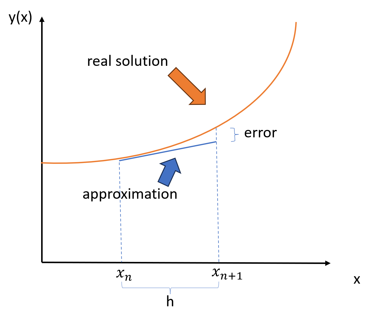
The Euler method offers a simple approach by breaking down the continuous ODE into discrete steps. The idea is to update the function's value based on its derivative at each step, effectively simulating the behavior of the ODE over a range of points. In fact, from any point $p$ on a curve, we can find an approximation of the nearby points on the curve by moving along the line tangent to $p$.
Let
$$\begin{equation} \begin{cases} \frac{\delta y}{\delta x}=f(x, y(x))\\ y(x_0)=y_0 \end{cases} \end{equation}$$
be our initial system.
Replacing the derivate with its discrete version and rearranging we get
$$\begin{equation} \begin{cases} y(x+h)=y(x) + h f(x, y(x))\\ y(x _0)=y_0 \end{cases} \end{equation}$$
and we can compute the following recursive scheme
$$y_{n+1}=y_n+hf(x_n,y_n)$$
Graphically:
Using the above equation, we can now compute \(y(x_n)\) \(\forall \space x_n\) with the following steps:
store \(y(x_0)=y_0\);
compute \(y(x_1)=y_0+hf(x_0, y_0)\);
store \(y(x_1)\);
compute \(y(x_2)=y_1+hf(x_1, y_1)\);
store \(y(x_2)\);
and so on.
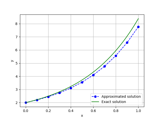
We now want to approximate the solution of the initial system
$$\begin{equation} \begin{cases} \frac{\delta y}{\delta x}=2y\\ y(0)=2 \end{cases} \end{equation}$$
and visualize the exact solution and the approximation
import numpy as np
import matplotlib.pyplot as plt

# define params, ode and inital condition
k = 2
f = lambda y, x: k*np.exp(k*y)
h = 0.1
x = np.arange(0, 1 + h, h)
x_= np.arange(0, 1, 0.0001)
y0 = 2

# initialize the y vector
y = np.zeros(len(x))
y[0] = y0

# populate the y vector
for i in range(0, len(x) - 1):
    y[i + 1] = y[i] + h*f(x[i], y[i])

# plot the results
plt.plot(x, y, 'bo--', label='Approximated solution')
plt.plot(x_, np.exp(k*x_)+1, 'g', label='Exact solution')
plt.xlabel('x')
plt.ylabel('y')
plt.grid()
plt.legend(loc='lower right')
plt.show()
Runge-Kutta methods
The Euler method is often not enough accurate. One solution is to use more than one point in the interval \([x_n, x_{n+1}]\) as the Runge-Kutta methods do. The number of points in the interval \([x_n, x_{n+1}]\) defines the order of the method.
Second-Order Runge-Kutta Method (RK2)
Starting with the Runge-Kutta method of order 2, we need the following second-order Taylor expansion:
$$y(x+h)=y(x)+h\frac{\delta y}{\delta x}(x) + \frac {h^2}2\frac{\delta^2 y}{\delta x^2}(x)+\epsilon$$
where \(\epsilon\) is the truncation error.
We can obtain \(\frac{\delta^2 y}{\delta x^2}(x)\) by differentiating the ODE \(\frac{\delta y}{\delta x}(x)=f(x, y(x))\):
$$\frac{\delta^2 y}{\delta x^2}(x)=\frac{\delta }{\delta x}f(x, y)+\frac{\delta}{\delta y}f(x, y)f(x, y)$$
and the Taylor expansion hence becomes
$$y(x+h)=y(x)+hf(x,y) + \frac {h^2}2(\frac{\delta }{\delta x}f(x, y)+\frac{\delta}{\delta y}f(x, y)f(x, y) )+\epsilon$$
After some manipulation, we obtain
$$y(x+h)=y(x)+\frac h2f(x,y) + \frac {h}2f(x+h,y+hf(x,y))+\epsilon$$
which corresponds to the following recursive scheme:
$$y_{n+1}=y_n+\frac h2(s_1+s_2)$$
with
$$s_1=f(x_n, y_n)\\$$
$$s_2 = f(x_n+\frac h2, y_n+\frac h2{s_1})$$
Note that \(s_1\) and \(s_2\) correspond to two different estimates of the slope of the solution and the method is nothing more than the average between the two.
Again using the above equation, we can compute \(y(x_n)\) \(\forall \space x_n\) with the following steps:
store \(y(x_0)=y_0\);
compute \(s_1 \) and \(s_2\);
compute \(y(x_1)=y_0+\frac h2(s_1+s_2)\);
store \(y(x_1)\);
update \(s_1 \) and \(s_2\);
\(y(x_2)=y_1+\frac h2(s_1+s_2)\);
store \(y(x_2)\);
and so on.
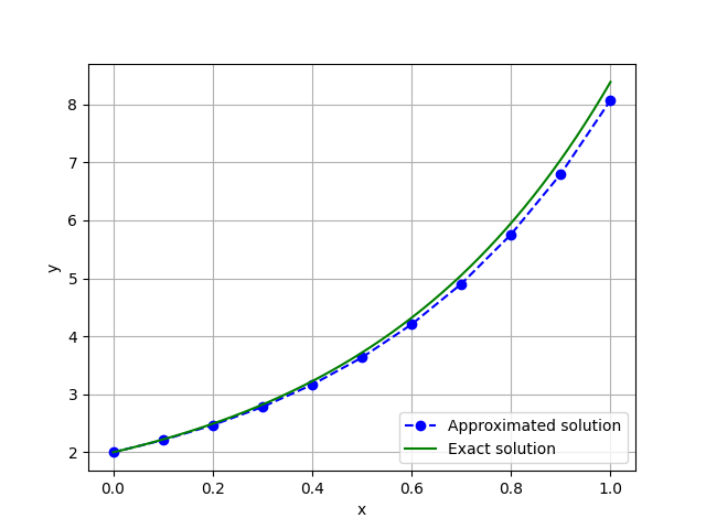
Again, we want to approximate the solution of the initial system
$$\begin{equation} \begin{cases} \frac{\delta y}{\delta x}=2y\\ y(0)=2 \end{cases} \end{equation}$$
import numpy as np
import matplotlib.pyplot as plt


# define params, the ode and the inital consition
k = 2
f = lambda y, x: k*np.exp(k*y)
h = 0.1
x = np.arange(0, 1 + h, h)
x_= np.arange(0, 1, 0.0001)
y0 = 2

# initialize thw y vector
y = np.zeros(len(x))
y[0] = y0

# populate the y vector
for i in range(0, len(x) - 1):
    s1=f(x[i], y[i])
    s2=f(x[i] + h/2, y[i]+  h/2*s1)
    y[i + 1] = y[i] + h/2 * (s1+s2)

# plot the results
plt.plot(x, y, 'bo--', label='Approximated solution')
plt.plot(x_, np.exp(k*x_)+1, 'g', label='Exact solution')
plt.xlabel('x')
plt.ylabel('y')
plt.grid()
plt.legend(loc='lower right')
plt.show()
Fourth-Order Runge-Kutta Method (RK4)
Repeating what we did to find the recursive scheme for the Range-Kutta method of order 2, but using a fourth-order Taylor expansion, we obtain the following recursive scheme:
$$y_{n+1}=y_n+\frac h3(\frac {s_1}2 + s_2 + s_3 + \frac{s_4}2)$$
with
$$s_1 = f(x_n, y_n)$$
$$s_2 = f(x_n+\frac h2, y_n+\frac h2{s_1})$$
$$s_3 = f(x_n+\frac h2, y_n+\frac h2{s_2})$$
$$s_4 = f(x_n+h, y_n+h{s_3})$$
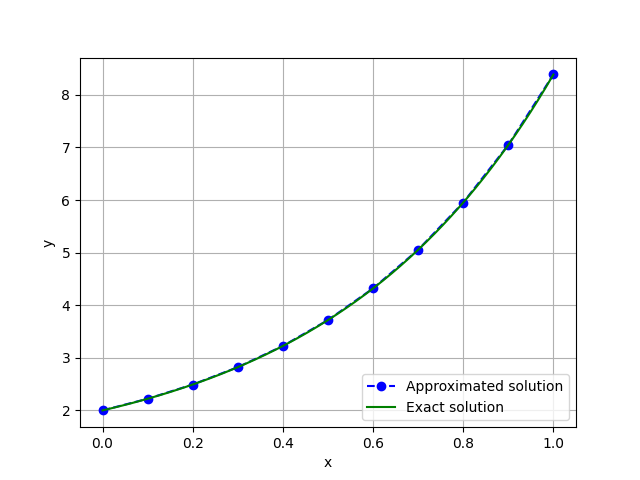
The steps used to approximate the system
$$\begin{equation} \begin{cases} \frac{\delta y}{\delta x}=2y\\ y(0)=2 \end{cases} \end{equation}$$
are specular to the ones used in the Runge-Kutta method of order 2.
import numpy as np
import matplotlib.pyplot as plt


# define params, the ode and the inital consition
k = 2
f = lambda y, x: k*np.exp(k*y)
h = .1
x = np.arange(0, 1 + h, h)
x_= np.arange(0, 1, 0.0001)
y0 = 2

# initialize thw y vector
y = np.zeros(len(x))
y[0] = y0

# populate the y vector
for i in range(0, len(x) - 1):
    s1=f(x[i], y[i])
    s2=f(x[i] + h/2, y[i]+  h/2*s1)
    s3=f(x[i] + h/2, y[i]+  h/2*s2)
    s4=f(x[i] + h, y[i]+  h*s3)
    y[i + 1] = y[i] + h/3 * (s1/2+s2+s3+s4/2)

# plot the results
plt.plot(x, y, 'bo--', label='Approximated solution')
plt.plot(x_, np.exp(k*x_)+1, 'g', label='Exact solution')
plt.xlabel('x')
plt.ylabel('y')
plt.grid()
plt.legend(loc='lower right')
plt.show()
There are also higher-order Range-Kutta methods but they are relatively inefficient, so I won't cover them in this article.
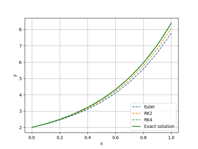
Comparison between the three methods
Euler Method:
Accuracy: the Euler method is a first-order method, which means that it can accumulate a significant error over many steps or for stiff ODEs.
Computational Complexity: the Euler method involves a single evaluation of the derivative function per step.
Second-Order Runge-Kutta Method (RK2):
Accuracy: RK2 is a second-order method: it offers better accuracy than the Euler method and is less prone to accumulating a relevant error over many steps.
Computational Complexity: RK2 requires two evaluations of the derivative function per step (one at the beginning and one at the midpoint).
Fourth-Order Runge-Kutta Method (RK4):
Accuracy: RK4 is a fourth-order method, which implies that it's significantly more accurate than both Euler and RK2 methods, making it suitable for many practical applications.
Computational Complexity: RK4 involves four evaluations of the derivative function per step, along with weighted combinations of these evaluations.
Despite the higher computational cost compared to Euler and RK2, RK4 still remains a popular choice due to its reliability and accuracy.
Graphically:
import numpy as np
import matplotlib.pyplot as plt

# define params, the ode and the inital consition
k = 2
f = lambda y, x: k*np.exp(k*y)
h = 0.1
x = np.arange(0, 1 + h, h)
x_= np.arange(0, 1, 0.0001)
y0 = 2

# initialize thw y vector
y = np.zeros(len(x))
y[0] = y0

# euler method
for i in range(0, len(x) - 1):
    y[i + 1] = y[i] + h*f(x[i], y[i])
plt.plot(x, y, label='Euler', linestyle='--')


# rk2 method
for i in range(0, len(x) - 1):
    s1=f(x[i], y[i])
    s2=f(x[i] + h/2, y[i]+  h/2*s1)
    y[i + 1] = y[i] + h/2 * (s1+s2)
plt.plot(x, y, label='RK2', linestyle='--')


# rk4 method
for i in range(0, len(x) - 1):
    s1=f(x[i], y[i])
    s2=f(x[i] + h/2, y[i]+  h/2*s1)
    s3=f(x[i] + h/2, y[i]+  h/2*s2)
    s4=f(x[i] + h, y[i]+  h*s3)
    y[i + 1] = y[i] + h/3 * (s1/2+s2+s3+s4/2)
plt.plot(x, y, label='RK4', linestyle='--')


plt.plot(x_, np.exp(k*x_)+1, label='Exact solution')
plt.xlabel('x')
plt.ylabel('y')
plt.grid()
plt.legend(loc='lower right')
plt.show()
And that's it for this article.
Thanks for reading.
For any question or suggestion related to what I covered in this article, please add it as a comment. For special needs, you can contact me here.