Simulated annealing in Python

Optimization is a crucial aspect of many fields, as it helps us find the best possible solution to a problem. In statistics, for example, it’s common to maximize the likelihood function or minimize the norm of residuals, in microeconomics optimization is used to study the behaviour of economic agents, who are assumed to maximize their utility subject to various constraints.
There are many different types of optimization problems, including linear programming, nonlinear programming, convex optimization, and integer programming, to name a few. Each type of optimization problem requires a different approach and a different set of algorithms to solve it.
In this post, I will talk about simulated annealing, which is a well-known algorithm but also is still exotic for noninitiated. For the sake of simplicity, I'll talk about minimization problems since seeking the maximum of a function $f$ equals seeking the maximum of a function \(-f\).
Simulated annealing
Simulated annealing is an iterative method for solving unconstrained and bound-constrained optimization problems. The algorithm borrows inspiration from the physical process of heating a material and then slowly lowering the temperature.
At each iteration of the simulated annealing algorithm, a new point \(x_i\) is randomly generated (if you don't know how computers deal with randomicity, see this article). As we'll see in a minute, the distance of the new point \(x\_i\) from the current point \(x\_{i-1}\) is proportional to the temperature and based on a certain probability distribution. The algorithm accepts all new points \(x_i \) such that \(f(x\_i) \leq f(x\_{i-1})\) where $f$ is the objective function (i.e. the function to be minimized), but also \(x_i \) such that \(f(x\_i) \geq f(x\_{i-1})\), with a certain probability. This property is significant and it prevents the algorithm from being trapped in local minima.
Simulated annealing with Python
First of all, we need to load some packages:
import math
import random as rd
We now define the parameters, we need:
an objective function $f$;
a domain (where the algorithm should look for a solution);
initial temperature;
an initial point (which is usually selected randomly);
a step size;
a maximum number of iterations.
# 1) the objective function
def f(x):
    return x**3 - 8

# 2) the domain
domain = [-10., 10.]

# 3) initial temperature
start_temp = 100

# 4) starting value
x_0 = rd.uniform(domain[0], domain[1])

# 5) the step size
step_size = 2

# 6) maximum number of iterations
max_iter = 1000
iteration = 0
First of all, we evaluate \(x_0\) and assign \(x_0\) and \(y_0 \) to x_best and y_best (the best value since now) and x_curr and y_curr (the current solution).
y_0 = f(x_0)

x_curr, y_curr = x_0, y_0
x_best, y_best = x_0, y_0
The first step of the algorithm is to generate a new candidate solution \(f(x_1) \) from the current solution \(f(x_0)\). We count an iteration (this step is crucial, otherwise the algorithm would run forever).
x_1 = x_curr + step_size * rd.uniform(-1, 1)
y_1 = f(x_1)

iteration += 1
Since we are looking for a minimum, if y_1 is smaller than y_best, we assign y_1 and x_1 to y_best and x_best. We then calculate the difference between y_best and y_curr.
if y_1 < y_best:
    x_best, y_best = x_1, y_1

diff = y_1 - y_curr
Here comes the most exciting part: we update the temperature (using fast annealing schedule) and use this value to calculate the Metropolis criterion:
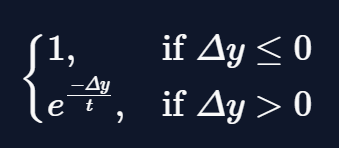
where \(\Delta y\) is diff and $t$ is temp. The numbers represent the probability of accepting the transition from \(x\_i\) to \(x\_{i+1}\) and are what allows to escape local minima.
temp = start_temp / (iteration + 1.)
metropolis = math.exp(-diff / temp)

if diff <= 0 or rd.random() < metropolis:
    x_curr, y_curr = x_best, y_best
And this is the last step. In fact after that, the algorithm calculates \(x_3\) and \(y_3\) and evaluates them for x_best and y_best and x_curr and y_curr and repeat itself until iteration == max_iter.
Making a function for simulated annealing
Since the algorithm at some point repeats itself, we may want to wrap it up in a function.
import math
import numpy as np
import random as rd

def simulated_annealing(f, domain, step_size, start_temp, max_iter = 1000):

    x_0 = rd.uniform(domain[0], domain[1])
    y_0 = f(x_0)
    x_curr, y_curr = x_0, y_0
    x_best, y_best = x_0, y_0

    for n in range(max_iter):
        x_i = x_curr + step_size * rd.uniform(-1, 1)
        y_i = f(x_i)

        if y_i < y_best:
            x_best, y_best = x_i, y_i

        diff = y_best - y_curr

        temp = start_temp/ float(n + 1)
        metropolis = math.exp(-diff / start_temp)

        if diff <= 0 or rd.random() < metropolis:
            x_curr, y_curr = x_i, y_i

    return [y_best, x_best]
Note that we don't have to count the iterations since we are using a for loop.
If we test the function we see that for well-chosen parameters the algorithm finds the value with a good approximation.
def fun(x):
    return x**2 + np.sin(x**4)

simulated_annealing(f = fun, domain = [-3, 3], step_size = 1, start_temp = 100, max_iter = 1000)

#> [9.915548806706291e-08, -0.00031488962865622305]
Finally, we plot what we got (the red line is the real minimum while the blue one is our result):
import numpy as np
from matplotlib import pyplot as plt

def fun(x):
    return x**2 + np.sin(x**4)

x = np.linspace(-3, 3, 1000)
y = fun(x)

plt.plot(x, y)

plt.axvline(x = 0, color = "blue", label = "real minimum")
plt.axvline(x = 9.915548806706291e-08, color = "red", label = "approximate minimum")
plt.legend(bbox_to_anchor = (1.0, 1), loc = "upper left")

plt.show()
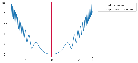
In the picture, the approximate minimum overlaps the real minimum (they are too close) and only the approximate minimum is visible.
Beyond 2D
Of course, the algorithm work also in more than one dimension, but the function needs some adjustment. In particular, we have to define a domain for y:
def simulated_annealing_3d(f, domain_x, domain_y, step_size, start_temp, max_iter = 1000):

    x_0 = rd.uniform(domain_x[0], domain_x[1])
    y_0 = rd.uniform(domain_y[0], domain_y[1])
    z_0 = f(x_0, y_0)
    x_curr, y_curr, z_curr = x_0, y_0, z_0
    x_best, y_best, z_best = x_0, y_0, z_0

    for n in range(max_iter):
        x_i = x_curr + step_size * rd.uniform(-1, 1)
        y_i = y_curr + step_size * rd.uniform(-1, 1)
        z_i = f(x_i, y_i)

        if z_i < z_best:
            x_best, y_best, z_best = x_i, y_i, z_i

        diff = z_i - z_curr

        temp = start_temp / (n + 1)
        metropolis = math.exp(-diff / temp)

        if diff <= 0 or rd.random() < metropolis:
            x_curr, y_curr, z_curr = x_i, y_i, z_i

    return [z_best, y_best, x_best]
Let's test the function:
def fun_3d(x, y):
    return (x-y)**2 + (x+y)**2

simulated_annealing_3d(f = fun_3d, domain_x = [-5, 5], domain_y = [-5, 5], step_size = 1, start_temp = 1000, max_iter = 10000)

#> [0.0007833147844967029, 0.018319454959260906, 0.007486986192318135]
If we plot the result:
from matplotlib import pyplot as plt

x = np.linspace(-.1, .1, 20)
y = np.linspace(-.1, .1, 20)
X, Y = np.meshgrid(x, y)
Z = fun_3d(X,Y)

a = np.repeat(0, 50)
b = np.repeat(0, 50)
c = np.arange(0, .05, .001)

a_ = np.repeat(0.015536251178558613, 50)
b_ = np.repeat(-0.014426988378332561, 50)
c_ = np.arange(0, .05, .001)

fig = plt.figure(figsize=(4,4))
ax = fig.add_subplot(111, projection='3d')
ax.plot_wireframe(X, Y, Z, color = "red", linewidth = .3)
ax.plot(a, b, c, color = "blue", label = "real minimum")
ax.plot(a_, b_, c_, color = "green", label = "approximated minimum")


ax.set_xlabel("x")
ax.set_ylabel("y")
ax.set_zlabel("z")
plt.legend(bbox_to_anchor = (1.0, 1), loc = "upper left")

plt.show()
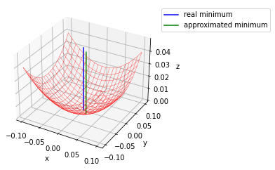
Zooming we can appreciate the error.
And that's it for this article.
Thanks for reading.
For any question or suggestion related to what I covered in this article, please add it as a comment. For special needs, you can contact me here.