Solving linear systems of equations using quantum computers

Linear systems of equations lie at the heart of many scientific and engineering problems, from machine learning to optimization and physics simulations. Classical methods like Gaussian elimination or iterative methods are powerful but can be inefficient for large, complex systems.
In this blog post, I will explore one of the most famous quantum algorithms (called HHL) that offer a potential speedup in solving linear systems. I will delve into its complexity, underlying assumptions and describe two interesting applications.
Quantum linear system problem versus linear system problem
In order to better understand the limitations of quantum algorithms like HHL, it’s essential to distinguish between a Quantum Linear System Problem (QLSP) and a classical Linear System Problem (LSP).
A typical linear system problem (LSP) is represented as:
$$Ax=b$$
where:
$A$ is a matrix
$b$ is a known vector
$x$ is the unknown vector we aim to solve for
On the other hand, a QLSP deals with a quantum state version of the same concept, represented as:
$$A\ket x = \ket b$$
where:
$A$ is still a matrix
\(\ket b\) is a known quantum state
\(\ket x\) is the unknown quantum state we wish to find
Although both problems appear similar, the difference lies in how the information is represented and manipulated. In a classical system, the vector $b$ is readily available, and solving for $x$ gives a concrete solution that can be directly used. In contrast, in the quantum setting, \(\ket b\) is a quantum state, and the solution \(\ket x\) is also a quantum state. The main challenge here is that quantum states aren’t directly accessible (any measurement of \(\ket x\) collapses the state and only provides a probabilistic result), which means that extracting useful information from the quantum solution requires multiple measurements or sophisticated post-processing.
Understanding these differences is crucial when assessing the complexity and feasibility of quantum solvers such as HHL, particularly when applied to real-world problems where error correction and measurement limitations play a significant role.
HHL
In this section, we introduce the Harrow-Hassidim-Lloyd (HHL) algorithm, one of the most interesting applications of the quantum phase estimation algorithm, which can be used to “solve” sparse linear linear systems, i.e. a system involving a matrix in which most of the elements are zero.
$$HHL: \ket b \rightarrow \ket {A^{-1}b}$$
In the next section the following assumptions will be true:
$A$ is a sparse and Hermitian matrix
the quantum state \(\ket b\) doesn’t have to be implemented from $b$
the problem requires to find \(\ket x\) instead of $x$
and the next section deal with:
the Quantum Phase Estimation algorithm
the workflow of HHL
complexity analysis of the HHL algorithm
what happens to the quantum advantage when the above assumptions fail to hold
a brief discussion of a couple of noteworthy applications of HHL
Please also note that many versions of the HHL algorithms have been proposed and this post only describe and deals with its simplest version.
Background: Quantum Phase Estimation
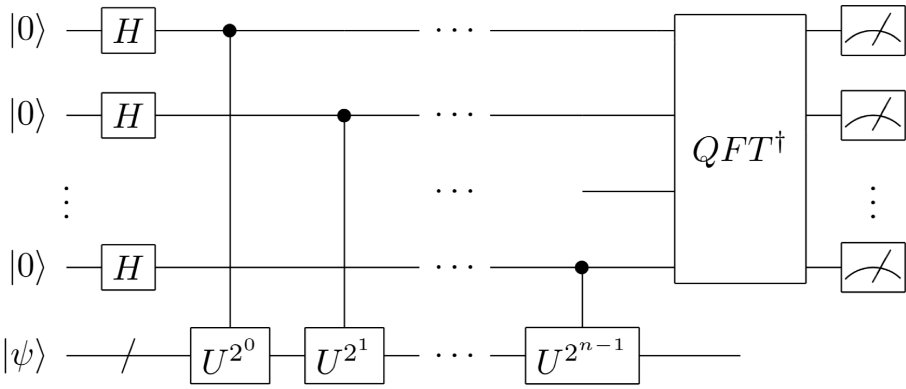
One of the most useful quantum subroutines, called Quantum Phase Estimation, aims to estimate the phase \(\phi\) of an eigenvalue \(e^{2i\pi\phi}\) of the corresponding eigenvector \(\ket \psi\)of a unitary operator $U$.

The QPE algorithm, depicted in the circuit above, shares similarities with Shor’s algorithm because Shor's algorithm can be seen as a specific application of QPE for integer factorization and the goal of QPE is to encode an estimation of the phase \(\phi\) into a binary representation like:
$$\phi = 0.\phi_1\phi_2\dots\phi_{n-1}\phi_n$$
QPE archive the result by phase encoding the binary representation of \(\phi\) using controlled $U$ gates in order to get the following state:
$$\left(\bigotimes_{j=1}^n \frac 1{\sqrt 2}(\ket 0 + e^{2i\pi0.\phi_j\dots \phi_n}\ket 1)\right) \otimes \ket\psi$$
and then applying the inverse of the Quantum Fourier Transform to go from the phase space to the state space and, before measuring, the result is:
$$\left(\bigotimes_{j=1}^n \ket {\phi_j}\right) \otimes \ket\psi = \ket {\hat \phi} \otimes \ket \psi$$
where \(\hat \phi\) is the estimation of \(\phi\).
HHL workflow

The above picture depicts the circuit of the HHL algorithm. One may notice that the algorithm can be broken down into 3 parts mainly:
a QPE
a controlled rotation
an inverse QFE
Assuming the input state \(\ket b\) is already prepared, the first block is used to find the phase of \(\{\lambda_i\}\) the eigenvalues of the matrix \(U = e^{i tA}\), and the approximated result is stored in the middle register.
At the end of the QPE, what we have is:
$$\ket 0 \otimes\left(\sum_i a_i \ket {u_i} \otimes \ket{\hat\lambda_i}\right)$$
where \(\sum_i a_i\ket {u_i}\) is \(\ket b\) expressed in terms of \(\ket {u_i}\), the eigenvalues of $U$ and \(\hat \lambda_i\) is the binary approximation of the phase of $U$.
Then a controlled rotation gate is applied, which corresponds to the following transformation:
$$\ket 0 \otimes\left( \sum_i a_i \ket {u_i} \otimes \ket{\hat\lambda_i}\right) \rightarrow \left(\sqrt{1-\left(\frac c\lambda\right)^2}\ket 0 + \frac c\lambda \ket 1\right)\otimes\left(\sum_i a_i \ket {u_i} \otimes \ket{\hat\lambda_i}\right)$$
where $c$ is a normalization constant.
The last block, the inverse QPE, is used to go from the state above to:
$$\ket q\otimes\left(\sum_i a_i \ket {u_i} \otimes \ket{\hat\lambda_i}\right) \rightarrow \ket q \otimes\left(\sum_i a_i \ket {u_i}\right)\otimes \ket{0}$$
where \(\ket q \equiv \left(\sqrt{1-\left(\frac c\lambda\right)^2}\ket 0 + \frac c\lambda \ket 1\right)\).
Notably, if the fist qubit (the top register) is measured we have two cases:
- if \(\ket q\) collapses into 1: once the middle register is measure as well, the result is:
$$∝\sum_i a_i \ket u_i \otimes \frac c{\lambda_i}$$
which is proportional to \(\ket {A^{-1}b}\) because of the spectral decomposition of $A$.
In fact \(A = \sum_i \lambda_i u_iu_i^\dagger\) and (by the properties of spectral decomposition) \(A^{-1} = \sum_i \lambda_i^{-1} u_iu_i^\dagger\) hence \(A^{-1}b = \sum_i a_i \lambda_i^{-1} u_i\) being \(u_i^\dagger u_i =1\) (for the properties of quantum states).
- if \(\ket q\) collapses into 0, one may run again the program
Complexity analysis
Let:
$k $ the conditional number (ratio of the largest and smallest absolute values of eigenvalues of $A$)
\(\epsilon \) the error from the output state \(\ket {A^{-1}b}\)
$s$ the maximum number of non-zero elements in each row of the matrix $A$
$N$ the size of the matrix
In fact, simulating \(e^{-iAt}\), if $A$ is $s$-sparse, can be done with error \(\epsilon\) in \(O(\log(N)s^2t\epsilon^{-1})\), which is required in the QPE process. One may then perform O(k) Quantum Amplitude Amplification repetitions to amplify the probability of measuring $1$, since \(C=O(\frac 1k)\) and if \(\lambda \leq 1\), the probability of measuring $1$ is \(\Omega(\frac 1{k^2})\).
Putting all together, then the computational complexity of the original HHL algorithm is:
$$O(\log(N)k^2s^2\epsilon^{-1})$$
however many improvements have been made and the computational complexity of the currently most efficient HHL algorithm is:
$$O\left(poly(\log(sk\epsilon^{-1}))sk\right )$$
and if we assume \(s = O(poly\left(\log(N)\right))\), the algorithm (focusing only on $N$) runs in:
$$O(poly\left(\log(N)\right))$$
which represents an exponential speedup in the matrix dimension compared to the best conjugate gradient method, whose complexity is:
$$O \left(Nsκlog\left(\frac 1\epsilon\right)\right)$$
However this holds on very specific assumptions and the next section deals with what happens if some of the assumptions are not met.
Loss of quantum advantage and near term feasibility of HHL
The computational complexity above, is based on the assumptions that:
\(\ket b\) is already available
doesn’t consider that \(\ket {A^{-1}b} \) should be read out
Note that if this input/output overhead takes $O(N)$, the exponential speedup is lost.
The computational cost of encoding $b$ in \(\ket b\) is:
$$O(N)$$
if $b$ is a simple bitstring and in general is:
$$O\left(2^N\right)$$
for a generic superposition, which results in the loss of the exponential speedup.
Moreover, also reading out the output solution state \(\ket {A^{-1}b}\) into a classical bitstring \(A^{-1}b\) requires $O(N)$, offsetting the exponential acceleration.
HHL in solving linear differential equations
One of the main applications of the HHL algorithm is solving linear differential equations. Quantum computers in fact can simulate quantum systems (which are described by a restricted type of linear differential equations), and using HHL it’s possible to solve general inhomogeneous sparse linear differential equations.
A first-order ordinary differential equation may be written as:
$$\frac {\delta x(t)}{\delta t}=A(t)x(t) + b(t)$$
where $A(t)$ is a \(N\times N\) matrix we assume to be sparse and $x(t)$ and $b(t)$ are $N$-components vectors.
A similar system can be the output of a conversion process from any linear differential equation with higher-order derivatives or from the discretization of partial differential equations.
A bunch of different methods involving HHL can be used to solve the above DE, however the workflow is roughly the same:
discretize the differential equation and get a system of algebraic equation
use HHL to find the solution of the system
In fact, one may apply a discretization scheme to the DE, for example the Euler method, to map the DE to a difference equation:
$$\frac{x_{i+1} + x_i}h= A(t_i)x_i + b(t_i)$$
and it is straightforward to see that this methods results in the following linear system:
$$Ax=b$$
where $x$ is the vector of blocks \(x_i\), and $b$ also contains the value of \(x_0\).
To learn more about this please see Berry, (2014), “High-order quantum algorithm for solving linear differential equations”.
HHL in solving least-square curve fitting
Another interesting application for HHL is least squares fitting. The goal in least squares fitting is to find a continuous function to approximate a discrete set of $N$ points \(\{x_i, y_i\}\). The function has to be linear in the parameter \(\theta \) but can be non linear in $x$, e.g.:
$$f(\theta, x) = \sum_i \theta_if_i(x)$$
The optimal parameters can be found by minimizing an error function such as the mean squared error:
$$E = |y - f(\theta, x)|^2$$
which can be expressed in matrix for as:
$$E= |y- F\theta|^2$$
where \(F_{ij}=f_j(x_i)\). The best fitting parameter can be found using Moore– Penrose pseudoinverse as:
$$\theta^* = \left(F^\dagger F\right)^{-1}F^\dagger y$$
Finding the best \(\theta\) then involves 3 subroutines:
performing the pseudo–inverse using the HHL algorithm and quantum matrix multiplication
an algorithm for estimating the fit quality
an algorithm for learning the fit-parameters \(\theta\)
To learn more about this please consider reading Wiebe, Brown, LLoyd, (2012), “Quantum Data-Fitting“.
And that's it for this article. Thanks for reading.
For any question or suggestion related to what I covered in this article, please add it as a comment. For special needs, you can contact me here.


