Physics informed neural networks for solving Partial Differential Equations

Introduction

Despite the grandiose name, Physics Informed Neural Networks (PINNs from now on) are simply neural networks trained to solve supervised learning tasks while adhering to any provided law of physics described by general nonlinear partial differential equations (PDEs from now on). The resulting neural network acts as a universal function approximator that inherently incorporates any underlying physical laws as prior knowledge, making them suitable for solving PDEs.

This not only signifies a stark departure from traditional numerical methods (such as finite difference, finite volume, finite elements, etc.) but also marks a shift in how we approach modeling and understanding physical systems. In fact, unlike conventional numerical techniques that depend on discretization and iterative solvers, PINNs offer a more comprehensive and data-centric approach and, by combining the capabilities of neural networks with the principles of physical laws, PINNs hold the potential to open up new pathways for exploration and innovation across various scientific fields.

In this blog post, my goal is to discuss all the essential components required to address PINNs for PDEs. Therefore, the post is composed of 4 key parts:

Firstly, I introduce PDEs and explain the necessity of relying on numerical methods;
Secondly, I provide a brief overview of neural networks;
Next, I delve into discussing PINNs;
Finally, I demonstrate how to implement PINNs using PyTorch.

About Partial Differential Equations (PDEs)

PDEs serve as fundamental tools in describing physical phenomena and natural processes across various scientific domains, from physics and engineering to biology and finance. Unlike ordinary differential equations (ODEs), which involve only one independent variable, PDEs incorporate multiple independent variables, such as space and time. For example

$$\frac{\delta f}{\delta t}+\alpha \frac{\delta f}{\delta x}=0$$

is known as the advection equation, where:

$f(t,x)$ is a function of two independent variables $x$ (space) and $t$ (time);
$\alpha$ is a constant;
$\frac{\delta f}{\delta t}$ represents the rate of change of $f$ with respect to time;
$\frac{\delta f}{\delta x}$represents the rate of change of $f$ with respect to space.

Physically, this equation describes how a quantity $f$ evolves over time $t$ as it is transported by a flow with constant speed $\alpha$ in the $x$-direction. In other words, it describes how $f$ moves along the $x$-axis with time, where the rate of change in time is proportional to the rate of change in space multiplied by the constant $\alpha$.

A closed form general solution to the advection function can be derived and corresponds to:

$$f(t,x)=g(x-at)$$

for any differentiable function $g(\cdot)$.

Not every PDE however admits a closed-form solution due to several reasons:

Complexity: many PDEs describe highly intricate physical phenomena with nonlinear behavior, making it difficult to find analytical solutions. Nonlinear PDEs, in particular, often lack closed-form solutions because of their intricate interdependence between variables;
Boundary conditions: solution to a PDE often depends not only on the equation itself but also on the boundary and initial conditions. If these conditions are complex or not well-defined, finding a closed-form solution becomes exceedingly challenging;
Non-standard formulation: some PDEs might be in non-standard forms that don't lend themselves easily to analytical techniques. For example, PDEs with non-constant coefficients or with terms involving higher-order derivatives may not have straightforward analytical solutions.
Inherent nature of the problem: certain systems are inherently chaotic or exhibit behaviors that resist simple mathematical description. For such systems, closed-form solutions may not exist, or if they do, they might be highly unstable or impractical.

For all the reasons mentioned, scientists usually depend on numerical methods to estimate the solution to PDEs (like PINNs, finite elements, finite volume, finite difference, and spectral method). In this post, I am only covering PINNs, while another post about other methods is on its way.

About neural networks

Once the problem that PINNs aim to solve is clear, we will now discuss some essential topics about neural networks. Since this is a very broad subject, I will only cover the most important aspects.

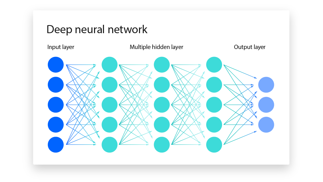
Neural networks are algorithms inspired by the workings of the human brain. In our brains, neurons process incoming data, such as visual information from our eyes, to recognize and understand our surroundings. Similarly, neural networks operate by receiving input data (input layer), processing it to identify patterns (hidden layer), and producing an output based on this analysis (output layer). Therefore, a neural network is typically represented as shown in the following picture:

Source: engineersplanet.com

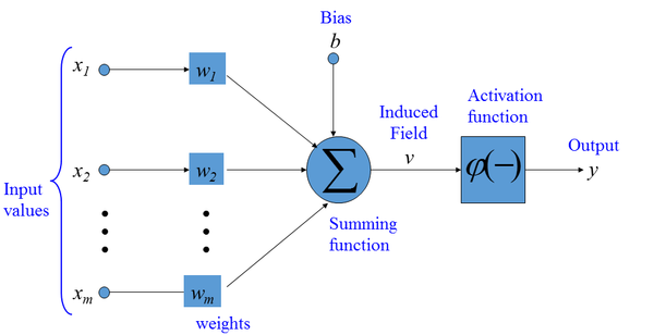
The basic unit of computation in a neural network is the neuron. It receives input from other nodes or an external source and calculates an output. Each input is linked with a weight (w, which the network learns), and every neuron has a unique input known as the bias (b), which is always set to 1. The output from the neuron is calculated as the weighted sum of the inputs, which is then sent to the activation function (introducing non-linearity into the output).

That said, a neural network comprises multiple interconnected neurons. While various architectures are tailored for specific issues, we will now concentrate on basic neural networks, also referred to as Feedforward neural networks (FNN).

Learning in neural networks

What is learnable in a neural networks are the weights and the bias and the learning process is divided in two parts:

feed forward propogation;
backward propogation.

In fact, learning occurs by adjusting connection weights after processing each piece of data, depending on the error in the output compared to the expected result.

Feedforward propagation

Feedforward propagation is the foundational process in neural networks where input data is processed through the layers to produce an output. This process is crucial for making predictions or classifications based on the given input. In feedforward propagation:

the flows in a unidirectional manner from the input layer through the hidden layers (if any) to the output layer;
each neuron in a layer receives inputs from all neurons in the previous layer. The inputs are combined with weights and a bias term, and the result is passed through an activation function to produce the neuron's output;
this process is repeated for each layer until the output layer is reached.

Backward propagation

Backward propagation, also known as backpropagation, is the process by which a neural network learns from its mistakes and adjusts its parameters (weights and biases) to minimize the difference between its predictions and the true targets. In backward propagation:

after the output is generated through feedforward propagation, the network's performance is evaluated using a loss function, which measures the difference between the predicted output and the true target values;
the gradient of the loss function with respect to each parameter (weight and bias) in the network is computed using the chain rule of calculus. This gradient indicates the direction and magnitude of the change needed to minimize the loss function;
the gradients are then used to update the parameters of the network in the opposite direction of the gradient, a process known as gradient descent. This update step involves adjusting the parameters by a small amount proportional to the gradient and a learning rate hyperparameter.

Neural networks as universal function approximators

Pivotal to Physics-Informed Neural Networks (PINNs) is a crucial theoretical concept concerning neural networks: their capability as universal function approximators. This fundamental property implies that neural networks can effectively approximate any continuous function with remarkable precision, given a sufficient number of neurons and an appropriate network configuration. Considering that the goal of PINNs is to estimate the solution to a Partial Differential Equation (PDE), which essentially involves approximating a function, this characteristic holds immense significance for the success and efficacy of PINNs in their predictive tasks.

About physics informed neural networks (PINNs)

Once the basics of deep learning are clear, we can delve deeper into understanding Physics Informed Neural Networks (PINNs).

Physics Informed Neural Networks (PINNs) serve as universal function approximators, with their neural network architecture representing solutions to specific Partial Differential Equations (PDEs). The core concept behind PINNs, as implied by their name, involves integrating prior knowledge about the system's dynamics into the cost function. This integration allows for penalizing any deviations from the governing PDEs by the network's solution.

Moreover, PINNs necessitate addressing the differences between the network's predictions and the actual data points within the cost function. This process is crucial for refining the network's accuracy and ensuring that it aligns closely with the observed data, thereby enhancing the model's predictive capabilities.

Therefore the loss function is:

$$\text{total loss} = \text{data loss + physics loss}$$

and (once a norm $|\cdot|$ is chosen) becomes:

$$\text{total loss} = \frac1n\sum |y_i - \hat y(x_i|\theta)| + \frac \lambda m\sum |f(x_j, \hat y(x_j|\theta))|$$

where:

$\hat y(x| \theta) $ is our neural network;
$x_i \text{ and } y_i$ are the data;
$f(x, g)=0$ is the PDE;
$\lambda$ is an hyperparameter.

and is equivalent to means squared error (MSE) when the chosen norm is the squared L2 norm.

Once we have this, we can train our PINN as a regular neural network.

A comparison between PINNs and classical methods

Compared to the traditional numerical simulation approaches, PINNs have the following desiderable properties:

PINNs are mesh-free, i..e they can handle complex domains, with a potential computational advantage;
PINNs are well-suited for modeling complex and nonlinear systems, because of the universa approximation theorem.

PyTorch implementation

This final section focuses on a PyTorch example to apply the theory in practice.

While this blog post mainly discussed PDEs, before approximating a PDE with a PINN, I aim to approximate an ODE using a PINN.

Approximating an ODE using a PINN: the logistic equation

The logistic equation is a differential equation used to model population growth in situations where resources are limited. It is often represented as:

$$\frac{dP}{dt} = rP\left(1 - \frac{P}{K}\right)$$

where:

$P$ represents the population size at time $t$;
$r$ is the intrinsic growth rate of the population;
$K$ is the carrying capacity of the environment, representing the maximum population size that the environment can sustain.

The analytical solution to the logistic equation is given by the logistic function:

$$P(t) = \frac{K}{1 + \left(\frac{K-P_0}{P_0}e^{-rt}\right)}$$

First of all we need a neural network architecture:

# code from https://github.com/EdgarAMO/PINN-Burgers/blob/main/burgers_LBFGS.py

import torch
import torch.nn as nn
import numpy as np
from random import uniform

class PhysicsInformedNN():
    def __init__(self, X_u, u, X_f):
        # x & t from boundary conditions:
        self.x_u = torch.tensor(X_u[:, 0].reshape(-1, 1),
                                dtype=torch.float32,
                                requires_grad=True)
        self.t_u = torch.tensor(X_u[:, 1].reshape(-1, 1),
                                dtype=torch.float32,
                                requires_grad=True)

        # x & t from collocation points:
        self.x_f = torch.tensor(X_f[:, 0].reshape(-1, 1),
                                dtype=torch.float32,
                                requires_grad=True)
        self.t_f = torch.tensor(X_f[:, 1].reshape(-1, 1),
                                dtype=torch.float32,
                                requires_grad=True)

        # boundary solution:
        self.u = torch.tensor(u, dtype=torch.float32)

        # null vector to test against f:
        self.null =  torch.zeros((self.x_f.shape[0], 1))

        # initialize net:
        self.create_net()
        #self.net.apply(self.init_weights)

        # this optimizer updates the weights and biases of the net:
        self.optimizer = torch.optim.LBFGS(self.net.parameters(),
                                    lr=1,
                                    max_iter=50000,
                                    max_eval=50000,
                                    history_size=50,
                                    tolerance_grad=1e-05,
                                    tolerance_change=0.5 * np.finfo(float).eps,
                                    line_search_fn="strong_wolfe")

        # typical MSE loss (this is a function):
        self.loss = nn.MSELoss()

        # loss :
        self.ls = 0

        # iteration number:
        self.iter = 0

    def create_net(self):
        """ net takes a batch of two inputs: (n, 2) --> (n, 1) """
        self.net = nn.Sequential(
            nn.Linear(2, 20), nn.Tanh(),
            nn.Linear(20, 20), nn.Tanh(),
            nn.Linear(20, 20), nn.Tanh(),
            nn.Linear(20, 20), nn.Tanh(),
            nn.Linear(20, 20), nn.Tanh(),
            nn.Linear(20, 20), nn.Tanh(),
            nn.Linear(20, 20), nn.Tanh(),
            nn.Linear(20, 20), nn.Tanh(),
            nn.Linear(20, 20), nn.Tanh(),
            nn.Linear(20, 1))

    def init_weights(self, m):
        if type(m) == nn.Linear:
            torch.nn.init.xavier_normal_(m.weight, 0.1)
            m.bias.data.fill_(0.001)

    def net_u(self, x, t):
        u = self.net( torch.hstack((x, t)) )
        return u

    def net_f(self, x, t):
        u = self.net_u(x, t)

        u_t = torch.autograd.grad(
            u, t, 
            grad_outputs=torch.ones_like(u),
            retain_graph=True,
            create_graph=True)[0]

        u_x = torch.autograd.grad(
            u, x, 
            grad_outputs=torch.ones_like(u),
            retain_graph=True,
            create_graph=True)[0]

        u_xx = torch.autograd.grad(
            u_x, x, 
            grad_outputs=torch.ones_like(u_x),
            retain_graph=True,
            create_graph=True)[0]

        f = u_t + (u * u_x) - (nu * u_xx)

        return f

    def plot(self):
        """ plot the solution on new data """

        import matplotlib.pyplot as plt
        from mpl_toolkits.axes_grid1 import make_axes_locatable

        x = torch.linspace(-1, 1, 200)
        t = torch.linspace( 0, 1, 100)

        # x & t grids:
        X, T = torch.meshgrid(x, t)

        # x & t columns:
        xcol = X.reshape(-1, 1)
        tcol = T.reshape(-1, 1)

        # one large column:
        usol = self.net_u(xcol, tcol)

        # reshape solution:
        U = usol.reshape(x.numel(), t.numel())

        # transform to numpy:
        xnp = x.numpy()
        tnp = t.numpy()
        Unp = U.detach().numpy()

        # plot:
        fig = plt.figure(figsize=(9, 4.5))
        ax = fig.add_subplot(111)

        h = ax.imshow(Unp,
                      interpolation='nearest',
                      cmap='rainbow', 
                      extent=[tnp.min(), tnp.max(), xnp.min(), xnp.max()], 
                      origin='lower', aspect='auto')
        divider = make_axes_locatable(ax)
        cax = divider.append_axes("right", size="5%", pad=0.10)
        cbar = fig.colorbar(h, cax=cax)
        cbar.ax.tick_params(labelsize=10)
        plt.show()

    def closure(self):
        # reset gradients to zero:
        self.optimizer.zero_grad()

        # u & f predictions:
        u_prediction = self.net_u(self.x_u, self.t_u)
        f_prediction = self.net_f(self.x_f, self.t_f)

        # losses:
        u_loss = self.loss(u_prediction, self.u)
        f_loss = self.loss(f_prediction, self.null)
        self.ls = u_loss + f_loss

        # derivative with respect to net's weights:
        self.ls.backward()

        # increase iteration count:
        self.iter += 1

        # print report:
        if not self.iter % 100:
            print('Epoch: {0:}, Loss: {1:6.3f}'.format(self.iter, self.ls))

        return self.ls

    def train(self):
        """ training loop """
        self.net.train()
        self.optimizer.step(self.closure)

if __name__ == '__main__' :

    nu = 0.01 / np.pi         # constant in the diff. equation
    N_u = 100                 # number of data points in the boundaries
    N_f = 10000               # number of collocation points

    # X_u_train: a set of pairs (x, t) located at:
        # x =  1, t = [0,  1]
        # x = -1, t = [0,  1]
        # t =  0, x = [-1, 1]
    x_upper = np.ones((N_u//4, 1), dtype=float)
    x_lower = np.ones((N_u//4, 1), dtype=float) * (-1)
    t_zero = np.zeros((N_u//2, 1), dtype=float)

    t_upper = np.random.rand(N_u//4, 1)
    t_lower = np.random.rand(N_u//4, 1)
    x_zero = (-1) + np.random.rand(N_u//2, 1) * (1 - (-1))

    # stack uppers, lowers and zeros:
    X_upper = np.hstack( (x_upper, t_upper) )
    X_lower = np.hstack( (x_lower, t_lower) )
    X_zero = np.hstack( (x_zero, t_zero) )

    # each one of these three arrays haS 2 columns, 
    # now we stack them vertically, the resulting array will also have 2 
    # columns and 100 rows:
    X_u_train = np.vstack( (X_upper, X_lower, X_zero) )

    # shuffle X_u_train:
    index = np.arange(0, N_u)
    np.random.shuffle(index)
    X_u_train = X_u_train[index, :]

    # make X_f_train:
    X_f_train = np.zeros((N_f, 2), dtype=float)
    for row in range(N_f):
        x = uniform(-1, 1)  # x range
        t = uniform( 0, 1)  # t range

        X_f_train[row, 0] = x 
        X_f_train[row, 1] = t

    # add the boundary points to the collocation points:
    X_f_train = np.vstack( (X_f_train, X_u_train) )

    # make u_train
    u_upper =  np.zeros((N_u//4, 1), dtype=float)
    u_lower =  np.zeros((N_u//4, 1), dtype=float) 
    u_zero = -np.sin(np.pi * x_zero)  

    # stack them in the same order as X_u_train was stacked:
    u_train = np.vstack( (u_upper, u_lower, u_zero) )

    # match indices with X_u_train
    u_train = u_train[index, :]

    # pass data sets to the PINN:
    pinn = PhysicsInformedNN(X_u_train, u_train, X_f_train)

    pinn.train()

Then we can build our loss function and define our ODE:

from typing import Callable
import argparse

import matplotlib.pyplot as plt
import torch
from torch import nn
import numpy as np
import torchopt

from pinn import make_forward_fn, LinearNN


R = 1.0  # rate of maximum population growth parameterizing the equation
X_BOUNDARY = 0.0  # boundary condition coordinate
F_BOUNDARY = 0.5  # boundary condition value


def make_loss_fn(f: Callable, dfdx: Callable) -> Callable:
    """Make a function loss evaluation function

    The loss is computed as sum of the interior MSE loss (the differential equation residual)
    and the MSE of the loss at the boundary

    Args:
        f (Callable): The functional forward pass of the model used a universal function approximator. This
            is a function with signature (x, params) where `x` is the input data and `params` the model
            parameters
        dfdx (Callable): The functional gradient calculation of the universal function approximator. This
            is a function with signature (x, params) where `x` is the input data and `params` the model
            parameters

    Returns:
        Callable: The loss function with signature (params, x) where `x` is the input data and `params` the model
            parameters. Notice that a simple call to `dloss = functorch.grad(loss_fn)` would give the gradient
            of the loss with respect to the model parameters needed by the optimizers
    """

    def loss_fn(params: torch.Tensor, x: torch.Tensor):

        # interior loss
        f_value = f(x, params)
        interior = dfdx(x, params) - R * f_value * (1 - f_value)

        # boundary loss
        x0 = X_BOUNDARY
        f0 = F_BOUNDARY
        x_boundary = torch.tensor([x0])
        f_boundary = torch.tensor([f0])
        boundary = f(x_boundary, params) - f_boundary

        loss = nn.MSELoss()
        loss_value = loss(interior, torch.zeros_like(interior)) + loss(
            boundary, torch.zeros_like(boundary)
        )

        return loss_value

    return loss_fn


if __name__ == "__main__":

    # make it reproducible
    torch.manual_seed(42)

    # parse input from user
    parser = argparse.ArgumentParser()

    parser.add_argument("-n", "--num-hidden", type=int, default=5)
    parser.add_argument("-d", "--dim-hidden", type=int, default=5)
    parser.add_argument("-b", "--batch-size", type=int, default=30)
    parser.add_argument("-lr", "--learning-rate", type=float, default=1e-1)
    parser.add_argument("-e", "--num-epochs", type=int, default=100)

    args = parser.parse_args()

    # configuration
    num_hidden = args.num_hidden
    dim_hidden = args.dim_hidden
    batch_size = args.batch_size
    num_iter = args.num_epochs
    tolerance = 1e-8
    learning_rate = args.learning_rate
    domain = (-5.0, 5.0)

    # function versions of model forward, gradient and loss
    model = LinearNN(num_layers=num_hidden, num_neurons=dim_hidden, num_inputs=1)
    funcs = make_forward_fn(model, derivative_order=1)

    f = funcs[0]
    dfdx = funcs[1]
    loss_fn = make_loss_fn(f, dfdx)

    # choose optimizer with functional API using functorch
    optimizer = torchopt.FuncOptimizer(torchopt.adam(lr=learning_rate))

    # initial parameters randomly initialized
    params = tuple(model.parameters())

    # train the model
    loss_evolution = []
    for i in range(num_iter):

        # sample points in the domain randomly for each epoch
        x = torch.FloatTensor(batch_size).uniform_(domain[0], domain[1])

        # compute the loss with the current parameters
        loss = loss_fn(params, x)

        # update the parameters with functional optimizer
        params = optimizer.step(loss, params)

        print(f"Iteration {i} with loss {float(loss)}")
        loss_evolution.append(float(loss))

    # plot solution on the given domain
    x_eval = torch.linspace(domain[0], domain[1], steps=100).reshape(-1, 1)
    f_eval = f(x_eval, params)
    analytical_sol_fn = lambda x: 1.0 / (1.0 + (1.0/F_BOUNDARY - 1.0) * np.exp(-R * x))
    x_eval_np = x_eval.detach().numpy()
    x_sample_np = torch.FloatTensor(batch_size).uniform_(domain[0], domain[1]).detach().numpy()

    fig, ax = plt.subplots()

    ax.scatter(x_sample_np, analytical_sol_fn(x_sample_np), color="red", label="Sample training points")
    ax.plot(x_eval_np, f_eval.detach().numpy(), label="PINN final solution")
    ax.plot(
        x_eval_np,
        analytical_sol_fn(x_eval_np),
        label=f"Analytic solution",
        color="green",
        alpha=0.75,
    )
    ax.set(title="Logistic equation solved with PINNs", xlabel="t", ylabel="f(t)")
    ax.legend()

    fig, ax = plt.subplots()
    ax.semilogy(loss_evolution)
    ax.set(title="Loss evolution", xlabel="# epochs", ylabel="Loss")
    ax.legend()

    plt.show()

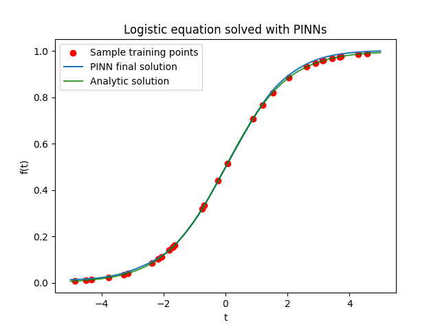
And this is the result:

Approximating a PDE using a PINN: the heat equation

The heat equation is a classical partial differential equation that describes the diffusion of heat (or equivalently, the distribution of temperature) in a given region over time. The one-dimensional form of the heat equation is given by:

$$\frac{\partial u}{\partial t} = \alpha \frac{\partial^2 u}{\partial x^2}$$

Again, we implement the PINN:

# code from https://github.com/udemirezen/PINN-1/blob/main/solve_PDE_NN.ipynb

import torch
import torch.nn as nn
from torch.autograd import Variable
device = torch.device("cuda:0" if torch.cuda.is_available() else "cpu")
import numpy as np

# We consider Net as our solution u_theta(x,t)

"""
When forming the network, we have to keep in mind the number of inputs and outputs
In ur case: #inputs = 2 (x,t)
and #outputs = 1

You can add ass many hidden layers as you want with as many neurons.
More complex the network, the more prepared it is to find complex solutions, but it also requires more data.

Let us create this network:
min 5 hidden layer with 5 neurons each.
"""

class Net(nn.Module):
    def __init__(self):
        super(Net, self).__init__()
        self.hidden_layer1 = nn.Linear(2,5)
        self.hidden_layer2 = nn.Linear(5,5)
        self.hidden_layer3 = nn.Linear(5,5)
        self.hidden_layer4 = nn.Linear(5,5)
        self.hidden_layer5 = nn.Linear(5,5)
        self.output_layer = nn.Linear(5,1)

    def forward(self, x,t):
        inputs = torch.cat([x,t],axis=1) # combined two arrays of 1 columns each to one array of 2 columns
        layer1_out = torch.sigmoid(self.hidden_layer1(inputs))
        layer2_out = torch.sigmoid(self.hidden_layer2(layer1_out))
        layer3_out = torch.sigmoid(self.hidden_layer3(layer2_out))
        layer4_out = torch.sigmoid(self.hidden_layer4(layer3_out))
        layer5_out = torch.sigmoid(self.hidden_layer5(layer4_out))
        output = self.output_layer(layer5_out) ## For regression, no activation is used in output layer
        return output
### (2) Model
net = Net()
net = net.to(device)
mse_cost_function = torch.nn.MSELoss() # Mean squared error
optimizer = torch.optim.Adam(net.parameters())
## PDE as loss function. Thus would use the network which we call as u_theta
def f(x,t, net):
    u = net(x,t) # the dependent variable u is given by the network based on independent variables x,t
    ## Based on our f = du/dx - 2du/dt - u, we need du/dx and du/dt
    u_x = torch.autograd.grad(u.sum(), x, create_graph=True)[0]
    u_t = torch.autograd.grad(u.sum(), t, create_graph=True)[0]
    pde = u_x - 2*u_t - u
    return pde
## Data from Boundary Conditions
# u(x,0)=6e^(-3x)
## BC just gives us datapoints for training

# BC tells us that for any x in range[0,2] and time=0, the value of u is given by 6e^(-3x)
# Take say 500 random numbers of x
x_bc = np.random.uniform(low=0.0, high=2.0, size=(500,1))
t_bc = np.zeros((500,1))
# compute u based on BC
u_bc = 6*np.exp(-3*x_bc)
### (3) Training / Fitting
iterations = 20000
previous_validation_loss = 99999999.0
for epoch in range(iterations):
    optimizer.zero_grad() # to make the gradients zero

    # Loss based on boundary conditions
    pt_x_bc = Variable(torch.from_numpy(x_bc).float(), requires_grad=False).to(device)
    pt_t_bc = Variable(torch.from_numpy(t_bc).float(), requires_grad=False).to(device)
    pt_u_bc = Variable(torch.from_numpy(u_bc).float(), requires_grad=False).to(device)

    net_bc_out = net(pt_x_bc, pt_t_bc) # output of u(x,t)
    mse_u = mse_cost_function(net_bc_out, pt_u_bc)

    # Loss based on PDE
    x_collocation = np.random.uniform(low=0.0, high=2.0, size=(500,1))
    t_collocation = np.random.uniform(low=0.0, high=1.0, size=(500,1))
    all_zeros = np.zeros((500,1))


    pt_x_collocation = Variable(torch.from_numpy(x_collocation).float(), requires_grad=True).to(device)
    pt_t_collocation = Variable(torch.from_numpy(t_collocation).float(), requires_grad=True).to(device)
    pt_all_zeros = Variable(torch.from_numpy(all_zeros).float(), requires_grad=False).to(device)

    f_out = f(pt_x_collocation, pt_t_collocation, net) # output of f(x,t)
    mse_f = mse_cost_function(f_out, pt_all_zeros)

    # Combining the loss functions
    loss = mse_u + mse_f


    loss.backward() # This is for computing gradients using backward propagation
    optimizer.step() # This is equivalent to : theta_new = theta_old - alpha * derivative of J w.r.t theta

    with torch.autograd.no_grad():
        print(epoch,"Traning Loss:",loss.data)

and then plot the result:

from mpl_toolkits.mplot3d import Axes3D
Axes3D = Axes3D
import matplotlib.pyplot as plt
from matplotlib import cm
from matplotlib.ticker import LinearLocator, FormatStrFormatter
import numpy as np

fig = plt.figure()
ax = fig.add_subplot(111, projection='3d')

x=np.arange(0,2,0.02)
t=np.arange(0,1,0.02)
ms_x, ms_t = np.meshgrid(x, t)
## Just because meshgrid is used, we need to do the following adjustment
x = np.ravel(ms_x).reshape(-1,1)
t = np.ravel(ms_t).reshape(-1,1)

pt_x = Variable(torch.from_numpy(x).float(), requires_grad=True).to(device)
pt_t = Variable(torch.from_numpy(t).float(), requires_grad=True).to(device)
pt_u = net(pt_x,pt_t)
u=pt_u.data.cpu().numpy()
ms_u = u.reshape(ms_x.shape)

surf = ax.plot_surface(ms_x,ms_t,ms_u, cmap=cm.coolwarm,linewidth=0, antialiased=False)

ax.zaxis.set_major_locator(LinearLocator(10))
ax.zaxis.set_major_formatter(FormatStrFormatter('%.02f'))

fig.colorbar(surf, shrink=0.5, aspect=5)

plt.show()

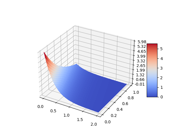
which returns the following:

And that's it for this article. Thanks for reading. If you have any suggestions for improvement or any further insights to share, please don't hesitate to reach out and leave a comment below. Your feedback is invaluable and greatly appreciated.

Physics informed neural networks for solving Partial Differential Equations

Comments

Numerical methods for differential equations

More from this blog

Quantum Principal Component Analysis and Self-Tomography

Post-Variational Quantum Neural Networks

Learning Parametric Partial Differential Equations using Fourier Neural Operator

Solving linear systems of equations using quantum computers

Computing Gradients of Quantum Circuits using Parameter Shift Rule

Introduction

About Partial Differential Equations (PDEs)

About neural networks

Learning in neural networks

Feedforward propagation

Backward propagation

Neural networks as universal function approximators

About physics informed neural networks (PINNs)

A comparison between PINNs and classical methods

PyTorch implementation

Approximating an ODE using a PINN: the logistic equation

Approximating a PDE using a PINN: the heat equation

Reference

Command Palette

Comments

Numerical methods for differential equations

More from this blog

Introduction

About Partial Differential Equations (PDEs)

About neural networks

Learning in neural networks

Feedforward propagation

Backward propagation

Neural networks as universal function approximators

About physics informed neural networks (PINNs)

A comparison between PINNs and classical methods

PyTorch implementation

Approximating an ODE using a PINN: the logistic equation

Approximating a PDE using a PINN: the heat equation

Reference