Quantum Boltzmann Machines

Quantum Boltzmann Machines (QBMs) are at the cutting edge of quantum machine learning, offering a novel extension of classical Boltzmann machines through the lens of quantum mechanics. These models take advantage of quantum principles to push the boundaries of what classical Boltzmann machines can achieve.
In this blog post, we'll explore the core concepts behind QBMs and investigate how they leverage the distinctive features of quantum computing to advance probabilistic modelling and learning and we'll examine how QBMs build on classical methods and the potential they hold for transforming data analysis and problem-solving in machine learning.
Classical Boltzmann Machines
Before diving into Quantum Boltzmann Machines (QBMs), it's useful to understand classical Boltzmann Machines (BMs) since QBMs are inspired by and build upon the concepts of classical BMs.
The concept of Boltzmann Machines was introduced by Geoffrey Hinton and Terrence Sejnowski in the mid-1980s and the model is named after the physicist Ludwig Boltzmann, whose work on statistical mechanics inspired the probabilistic framework of the BM.
The impact of Boltzmann Machines has been broad and significant, for example in image and speech recognition, Restricted Boltzmann Machines (RBMs, an evolution of BMs) have excelled at unsupervised feature learning, improving classification accuracy. In recommendation systems, they’ve been used to predict user preferences and RMBs applications extend also to natural language processing for learning text representations and robotics for sensor fusion, combining data from multiple sources.
Classical architectures
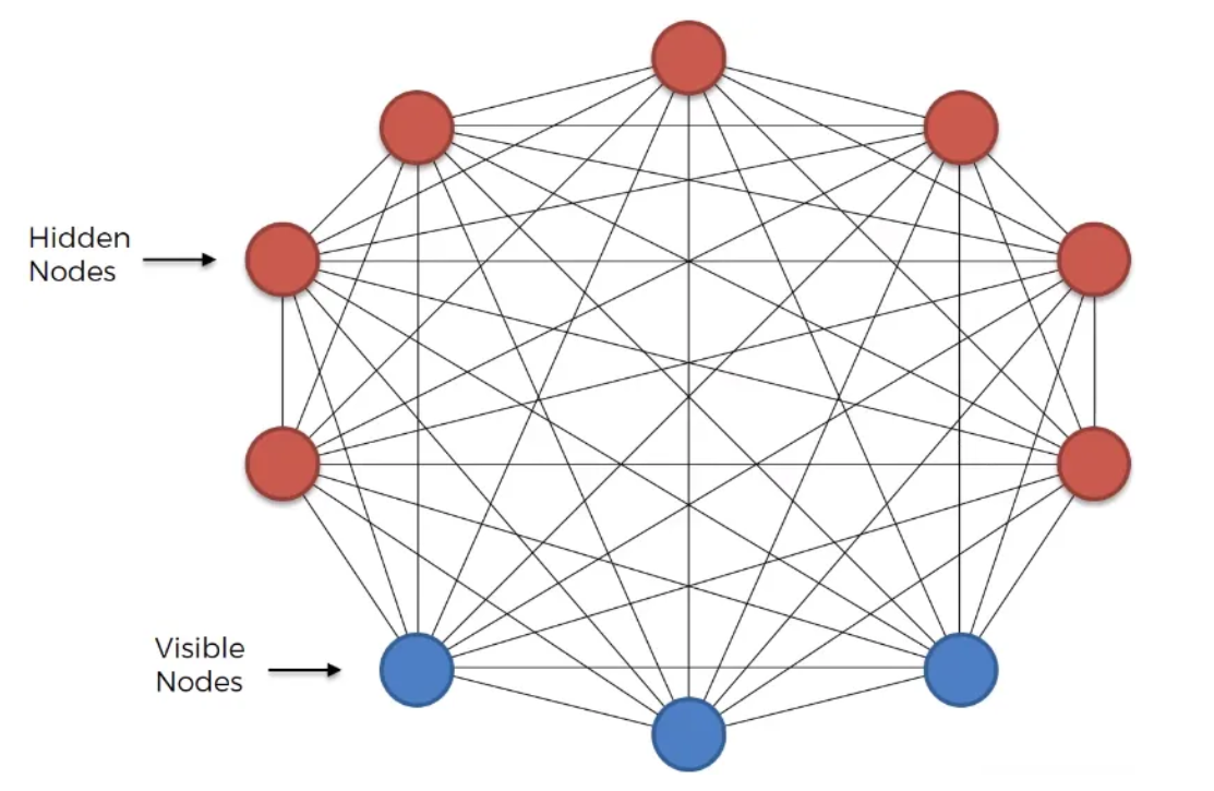
Basically, a Boltzmann Machine consists of a collection of binary units, also known as neurons, organized into two layers: visible units and hidden units. The visible units represent the observed variables, while the hidden units capture the latent or hidden variables that explain the relationships in the data.
Due to the exponential growth in the number of connections with an increase in nodes in a classical Boltzmann Machine (BM), the Restricted Boltzmann Machine (RBM) is often preferred. The RBM simplifies the architecture by restricting connections:
Hidden nodes are not connected to each other
Visible nodes are also not connected to each other
In RBMs, connections exist only between visible and hidden nodes, which makes the network more manageable and easier to train compared to the fully connected structure of classical BMs.
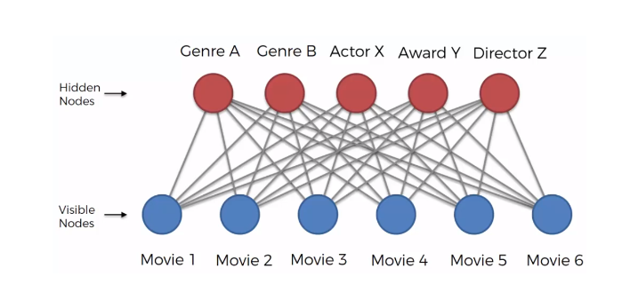
The objective of Boltzmann Machines is to model a probability distribution over a set of binary variables (units) in a way that captures the complex relationships and dependencies between these variables. This is achieved through the concept of energy.
The idea behind the energy based learning lies in the energy function, defined as
$$E(v, h) = - \sum_{i} b_i v_i - \sum_{j} c_j h_j - \sum_{i,j} W_{ij} v_i h_j$$
where:
\(b_i\) is the bias of the i-th visible node
\(v_i\) is the i-th visible node
\(c_j\) is the bias of the j-th hidden node
\(h_j\) is the j-th hidden node
\(W_{ij}\) is the weight of the connection between visible i-th unit and j-th hidden unit
To each configuration (\(v, \space h\)) a probability is assigned according to the following function:
$$P(v, h) = \frac{e^{-E(v, h)}}{\sum_{v, h} e^{-E(v, h)}}$$
and the goal is to minimizing the difference between the distribution defined by the BM and the true data distribution, i.e. to maximize the likelihood of the training data under the model:
$$\mathcal{L} = \sum_{v} P_{\text{data}}(v) \log P_{\text{model}}(v)$$
Training
In Boltzmann Machines, error adjustment cannot be achieved using a gradient descent process like in traditional neural networks, where weights are adjusted by backpropagating the error through the network. This is because BMs are undirected networks, meaning there is no distinction between input and output layers. As a result, BMs lack the concept of "backpropagation" since there is no directed flow of information to guide the adjustment of weights.
In fact, the algorithm typically used to train BMs is called Contrastive Divergence and is completely different in nature from backpropagation, since it approximates the gradient of the log-likelihood function by using a technique involving Gibbs sampling.
The algorithm is an iterative algorithm made by the following 2 steps:
Perform Gibbs sampling to approximate the distribution of the hidden and visible units based on their conditional probabilities
Compute the gradient and update the weights.
Gibbs sampling
Given a set of variables \(X=\{X_1, \dots X_n\}\) Gibbs sampling aims to sample from the joint distribution $P(X)$ which sometimes can be challenging, Therefore Gibbs sampling uses the conditional distributions \(P(X_i|X_{/i})\) where \(X_{/i}\) denotes all the variables except \(X_{i}\).
Therefore using this technique
$$X_i^{(t+1)} \sim P(X_i \mid X_1^{(t)}, X_2^{(t)}, \ldots, X_{i-1}^{(t)}, X_{i+1}^{(t)}, \ldots, X_n^{(t)})$$
In the context of BMs this translates to sampling the hidden units as
$$P(h_j = 1 \mid v) = \sigma \left( \sum_{i} W_{ij} v_i + c_j \right)$$
and the visible units as
$$P(v_i = 1 \mid h) = \sigma \left( \sum_{j} W_{ij} h_j + b_i \right)$$
where \(\sigma(x) = \frac{1}{1 + \exp(-x)}\).
Compute the gradient and update the weights
The gradient is then computed as:
$$\frac{\partial \mathcal{L}}{\partial W_{ij}} = \frac{\partial}{\partial W_{ij}} \left( \sum_{v} P_{\text{data}}(v) \log P_{\text{model}}(v) \right)$$
which, after some calculations results in:
$$\frac{\partial \mathcal{L}}{\partial W_{ij}} = \langle v_i h_j \rangle_{\text{data}} - \langle v_i h_j \rangle_{\text{model}}$$
where:
\(\langle v_i h_j \rangle_{\text{model}} = \sum_{v, h} P_{\text{model}}(v, h) v_i h_j\)
\(\langle v_i h_j \rangle_{\text{data}} = \sum_{v} P_{\text{data}}(v) v_i h_j\)
And the weights are updated iteratively as:
$$W_{ij}^{t+1} = W_{ij}^{t}+\epsilon \left( \langle v_i h_j \rangle_{\text{data}} - \langle v_i h_j \rangle_{\text{model}} \right)$$
where \(\epsilon\) is the learning rate.
Quantum Boltzmann machines
The concept of leveraging quantum mechanics for machine learning tasks has seen significant advancements over the past decade, with the Quantum Boltzmann Machine (QBMs) emerging as one of the results of these studies. In particular Mohammad Amin, Evgeny Andriyash, Jason Rolfe, Bohdan Kulchytskyy, and Roger Melko, arxiv:1601.02036 (2016) has developed a quantum probabilistic model based on Boltzmann distribution of a quantum Hamiltonian, which exploits quantum effects both in the model and in the training process.
The problem QBMs is exactly the same as BMs: finding the biases and weights parameters that better approximate a sample distribution by maximizing the log-likelihood, as defined above.
Quantum architecture
As for classical Boltzmann Machines, our treatment of QBMs starts from the energy function:
$$E(\xi) = -\sum_{i} \xi_i \beta_i - \sum_{i,j} W_{ij} \xi_i \xi_j$$
where:
- \(\xi_i\) represents a node (hidden or visible) which is a \(2^n \times 2^n\) matrix defined as ($I$is the identity matrix, \(\sigma_z\) is Pauli Z matrix, $N$ is the number of nodes):
$$\xi_i \equiv \overbrace{I \otimes \ldots \otimes I}^{i-1} \otimes \sigma_i^z \otimes \overbrace{I \otimes \ldots \otimes I}^{N-i}$$
- \(\beta\) represents the biases (for both hidden and visible nodes)
Using the energy function we define the Boltzmann distribution as:
$$P(\xi) = \frac{e^{-E(\xi)}}{\sum e^{-E(\xi)}}$$
where the matrix exponentiation is defined trough Taylor expansion:
$$e^{- E(\xi)}=\sum_{k=0}^{\infty} \frac{1}{k!}\left( - E(\xi) \right) ^k$$
Let also the partition function $Z$ be:
$$Z=Tr[e^{-E(\xi)}]$$
then the density matrix is:
$$\rho = Z^{-1}e^{-E(\xi)}$$
which represents the Boltzmann probability of the \(2^N\) elements. Therefore to get the marginal probability distribution over the visible variables \(\ket v\) we just need to trace over the hidden variables, i.e.:
$$P_v = Tr[(\ket v \bra v \otimes I_h)\rho]$$
which is the analogous of:
$$P(v, h) = \frac{e^{-E(v, h)}}{\sum_{v, h} e^{-E(v, h)}}$$
At this point, if we include in the Hamiltonian a new element representing a transverse field defined as:
$$\nu_i \equiv \overbrace{I \otimes \ldots \otimes I}^{i-1} \otimes \sigma_i^x \otimes \overbrace{I \otimes \ldots \otimes I}^{N-i}$$
where \(\sigma_x\) is the Pauli X matrix, the resulting Hamiltonian is:
$$E(\xi, \nu) = -\sum_{i} \xi_i \beta_i - \sum_{i,j} W_{ij} \xi_i \xi_j -\sum_i \Gamma_i\nu_i$$
where \(\Gamma_i\) is a parameter.
This new Hamiltonian is special since every eigenstate of \( E(\xi, \nu)\) is a superposition of the classical states \(\ket{v, h}\). Hence using the following density matrix defined above with this new Hamiltonian, each measurement in the \(\sigma_z\) basis results in a classical output in \( \{1, -1\}\), and the probability of each output is given by \(P_v\).
Training
As in the classical formulation, the scope of QMBs is to find the $W$ and $b$ (from now on I'm referencing these parameters as \(\theta\)) so that \(P_v\) (what before was called \(P_{\text{model}}\)) is close to \(P_\text{data}\).
Again this is achieved by minimizing the negative log-likelihood \(\mathcal{L}\):
$$\mathcal{L}=-\sum_{\mathbf{v}} P_{\text {data }} \log \frac{\operatorname{Tr}\left[(\ket v \bra v \otimes I_h) e^{-E(\xi, \nu)}\right]}{\operatorname{Tr}\left[e^{-E(\xi, \nu)}\right]}$$
whose gradient is:
$$\partial_\theta \mathcal{L}=\sum_{\mathbf{v}} P_{\text {data }}\left(\frac{\operatorname{Tr}\left[(\ket v \bra v \otimes I_h) \partial_\theta e^{-E(\xi, \nu)}\right]}{\operatorname{Tr}\left[(\ket v \bra v \otimes I_h) e^{-E(\xi, \nu)}\right]}-\frac{\operatorname{Tr}\left[\partial_\theta e^{-E(\xi, \nu)}\right]}{\operatorname{Tr}\left[e^{-E(\xi, \nu)}\right]}\right)$$
Ideally we would use some sampling techniques to estimate efficiently the gradient, however, since \(E(\xi, \nu)\) and \(\partial_\theta E(\xi, \nu)\) don't commute, we don't have a trivial solution.
In fact one can prove that:
$$\frac{\operatorname{Tr}\left[\partial_\theta e^{-E(\xi, \nu)}\right]}{\operatorname{Tr}\left[e^{-E(\xi, \nu)}\right]}= - \operatorname{Tr}[\rho {\partial_\theta}{E(\xi, \nu)}]$$
and that:
$$\frac{\operatorname{Tr}\left[(\ket v \bra v \otimes I_h) \partial_\theta e^{-E(\xi, \nu)}\right]}{\operatorname{Tr}\left[(\ket v \bra v \otimes I_h) e^{-E(\xi, \nu)}\right]}=-\int_0^1 d t \frac{\operatorname{Tr}\left[(\ket v \bra v \otimes I_h) e^{-t E(\xi, \nu)} \partial_\theta E(\xi, \nu)e^{-(1-t) E(\xi, \nu)}\right]}{\operatorname{Tr}\left[(\ket v \bra v \otimes I_h)e^{-E(\xi, \nu)}\right]}$$
and it can be shown that, while the first term can be estimated efficiently, the second one cannot be efficiently estimated using sampling, which makes the computational cost of training QBMs impractical. Is this the end of the story? Actually no, since the introduction of an upper bound on the \(\mathcal{L} \) (which is a common practice in machine learning) results in the so-called bound-based Quantum Boltzmann Machines (BQBMs), that provides a work around to the computational impracticability of QBMs, as discussed in next section.
Bound-based Quantum Boltzmann Machines
A very famous inequality, called Golden-Thompson inequality states that for any Hermitian matrix $A$ and $B$ the following is true:
$$\operatorname{Tr}\left( e^Ae^B\right) \geq \operatorname{Tr}\left( e^{A+B}\right)$$
Therefore we know that:
$$P_v = \frac{\operatorname{Tr}[e^{\log{(\ket v \bra v \otimes I_h)}}e^{-E(\xi, \nu)}]}{\operatorname{Tr}[e^{-E(\xi, \nu)}]} \geq \frac{\operatorname{Tr}[e^{H_\xi}]}{\operatorname{Tr}[e^{-E(\xi, \nu)}]}$$
where \(H_\xi \equiv \log{(\ket v \bra v \otimes I_h)}-E(\xi, \nu)\) and is a peculiar Hamiltonian since it assigns an infinite energy penalty for any state s.t. the visible qubits register is different from \(\ket v\). Mathematically, this means that the probability of the system being in any state other than \(\ket v\) is zero because the Boltzmann factor approaches zero for infinite energy.
This means, in other words, that every qubits \(\xi_i\) is clamped to the corresponding classical value \(v_i\).
From the Golden-Thompson inequality we can also derive that:
$$\mathcal{L} \le \hat{\mathcal{L}} \equiv \sum P_\text{data} \log \frac{\operatorname{Tr}[e^{H_\xi}]}{\operatorname{Tr}[e^{-E(\xi, \nu)}]}$$
and we can now minimize \(\hat{\mathcal L}\), the upper bound of \({\mathcal L}\), using the gradient and we get the following rules to update the bias \(\beta_i\):
$$\beta_i^{t+1}= \beta_i^{t} + \epsilon \left(\sum P_\text{data} \frac{\operatorname{Tr}[e^{-H_\xi}]\sigma_i^z}{\operatorname{Tr}[e^{-H_\xi}]} - \operatorname{Tr}(\rho \sigma_i^z)\right)$$
and the weight \(w_{ij}\):
$$W_{ij}^{t+1}= W_{ij}^{t} + \epsilon \left(\sum P_\text{data} \frac{\operatorname{Tr}[e^{-H_\xi}]\sigma_i^z\sigma_j^z}{\operatorname{Tr}[e^{-H_\xi}]} - \operatorname{Tr}(\rho \sigma_i^z\sigma_j^z)\right)$$
One may also think about training the \(\Gamma\), however this results in vanishing \(\Gamma\)i.e. learning the transverse field is unfeasible in this upper bound setting.
Semi-restricted Quantum Boltzmann Machines
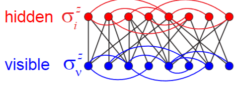
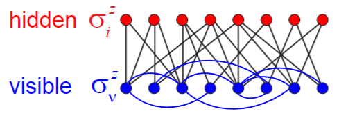
Untill now we never posed any restrictions on the structure of the QBM, and in particular we assumed a fully connected architecture. Similarly to classical RBMs, semi-restricted Quantum Boltzmann Machines (srQBMs) are quantum neural networks similar to QBMs whose hidden layer has lateral connectivity.
Note that, unlike classical RBMs, we are assuming the lateral connection in the only in the hidden layer.
A similar architecture in fact allows us to apply contrastive divergence learning algorithms since the clamped Hamiltonian is then:
$$H_\xi = - \sum_i \left(\Gamma_i \sigma_i^x + (b_i+ \sum_j W_{ij} v_j)\sigma_i^z \right)$$
as the hidden qubits are uncoupled during the parameters learning phase.
Based on the Hamiltonian one can show that expectations can be computed efficiently as:
$$\frac{\operatorname{Tr}[e^{-H_\xi}]\sigma_i^z}{\operatorname{Tr}[e^{-H_\xi}]}= \frac{b_i+ \sum_j W_{ij} v_j}{\sqrt{\Gamma_i^2 + (b_i+ \sum_j W_{ij} v_j)^2}}$$
which is equivalent to the classical RBMs expression as \(\Gamma_i \rightarrow 0\).
Conclusion
While being still experimental, Quantum Boltzmann Machines represent an exciting advancement in the field of quantum machine learning and the journey towards fully realizing the potential of Quantum Boltzmann Machines is ongoing, requiring collaboration across disciplines and continuous innovation. While it is important to temper expectations with the recognition of current limitations, the foundational work being done is not just an academic exercise but a step towards unlocking new possibilities in science and industry.
And that's it for this article. Thanks for reading.
For any question or suggestion related to what I covered in this article, please add it as a comment. For special needs, you can contact me here.
Sources
Mohammad Amin, Evgeny Andriyash, Jason Rolfe, Bohdan Kulchytskyy, and Roger Melko, arxiv:1601.02036 (2016)
G. E. Hinton, S. Osindero, Y-W. Teh, A fast learning algorithm for deep belief nets, Neural Comput. 18, 1527– 1554 (2006)
R. Salakhutdinov, G. E. Hinton, Deep Boltzmann machines, AISTATS 2009
Miguel Carreira-Perpinan, Geoffrey Hinton, On Contrastive Divergence Learning (2005)
